DifferentialEquations.jl v7: New linear solver and preconditioner interface
An update is long overdue and this is a really nice one! DifferentialEquations.jl v7 has been released, the first major version since 2019! We note that, as a major version, this does indicate breaking API changes have been introduced. That said, they are relatively minor and only involve the linear solver interface, which is the main topic of this release post.
Before we move on, I want to mention that all of your support helps. Thank you very much! If you do not have anything to donate, you can still help by starring the DifferentialEquations.jl and other Github repositories in the SciML Organization. If you do have funds, please consider becoming a sponsor. The next set of tools, like tutorials showing large sparse PDEs solved using Distributed and GPUs, will require support from viewers like you. Now back to the show.
LinearSolve.jl: A common interface for linear solvers
Julia has built in linear solvers, so why does this library exist? The problem is that the person who writes a library may not be the person who can make the best choice for how a linear system is solved. Thus while A\b looks like the "best" way to solve Ax=b, in reality there are many ways to do it:
lu(A)\bis the fastest of the factorizations for standard matrices, but if the matrix is positive definite thencholesky(A)\bcan be faster, etc. And if the matrix is ill-conditioned thenqr(A)\bwill have less numerical error.When you get to sparse arrays, there are many different LU-factorizations, like KLU.jl as an alternative to the standard UMFPACK one, which will be better or worse depending on the sparsity pattern.
There are methods which do not require constructing the full
Amatrix, like IterativeSolvers.jl or Krylov.jl Krylov-subspace methods. These cannot be represented by a simple\because they require specifying a tolerance.
Thus, how can you write a library but expose the linear solver choice to the user? The answer is LinearSolve.jl. Let's see it in action. Solve Ax=b with the default method:
using LinearSolve

A = rand(4,4)
b = rand(4)
prob = LinearProblem(A, b)
sol = solve(prob)
sol.u
Now let's choose an LU-factorization:
sol = solve(prob,LUFactorization())And now what about using GMRES with a relative tolerance of 1e-7?
sol = solve(prob,KrylovJL_GMRES(),reltol=1e-7)Notice this all follows the SciML Common Interface and thus has the same look and feel as NonlinearSolve.jl, DifferentialEquations.jl, and GalacticOptim.jl. There are many nice features in there, such as an iterative interface that helps with caching factorizations effectively. Thus for someone interesting in writing libraries which internally use linear solvers, this is a very nice target. In fact, that may be its main purpose, leading us to the next point.
LinearSolve.jl Integration into DifferentialEquations.jl
The major breaking change of DifferentialEquations.jl v7 is the use of LinearSolve.jl for internal linear solves. Now, linear solvers for implicit algorithms are chosen by passing a LinearSolve.jl solver to the linsolve of compatible OrdinaryDiffEq.jl algorithms. This is all showcased in the new and improved scaling stiff ODE solvers for PDEs tutorial
For example, let's say we are solving this big Brusselator PDE:
using DifferentialEquations, LinearAlgebra, SparseArrays

const N = 32
const xyd_brusselator = range(0,stop=1,length=N)
brusselator_f(x, y, t) = (((x-0.3)^2 + (y-0.6)^2) <= 0.1^2) * (t >= 1.1) * 5.
limit(a, N) = a == N+1 ? 1 : a == 0 ? N : a
function brusselator_2d_loop(du, u, p, t)
  A, B, alpha, dx = p
  alpha = alpha/dx^2
  @inbounds for I in CartesianIndices((N, N))
    i, j = Tuple(I)
    x, y = xyd_brusselator[I[1]], xyd_brusselator[I[2]]
    ip1, im1, jp1, jm1 = limit(i+1, N), limit(i-1, N), limit(j+1, N), limit(j-1, N)
    du[i,j,1] = alpha*(u[im1,j,1] + u[ip1,j,1] + u[i,jp1,1] + u[i,jm1,1] - 4u[i,j,1]) +
                B + u[i,j,1]^2*u[i,j,2] - (A + 1)*u[i,j,1] + brusselator_f(x, y, t)
    du[i,j,2] = alpha*(u[im1,j,2] + u[ip1,j,2] + u[i,jp1,2] + u[i,jm1,2] - 4u[i,j,2]) +
                A*u[i,j,1] - u[i,j,1]^2*u[i,j,2]
    end
end
p = (3.4, 1., 10., step(xyd_brusselator))

function init_brusselator_2d(xyd)
  N = length(xyd)
  u = zeros(N, N, 2)
  for I in CartesianIndices((N, N))
    x = xyd[I[1]]
    y = xyd[I[2]]
    u[I,1] = 22*(y*(1-y))^(3/2)
    u[I,2] = 27*(x*(1-x))^(3/2)
  end
  u
end
u0 = init_brusselator_2d(xyd_brusselator)
prob_ode_brusselator_2d = ODEProblem(brusselator_2d_loop,u0,(0.,11.5),p)
We can first speed it up by using the automated sparsity detection of Symbolics.jl to generate a sparse Jacobian:
using Symbolics
du0 = copy(u0)
jac_sparsity = Symbolics.jacobian_sparsity((du,u)->brusselator_2d_loop(du,u,p,0.0),du0,u0)

2048×2048 SparseArrays.SparseMatrixCSC{Bool, Int64} with 12288 stored entries:
⠻⣦⡀⠀⠀⠀⠀⠈⠳⣄⠀⠀⠀⠀⠀⠀
⠀⠈⠻⣦⡀⠀⠀⠀⠀⠈⠳⣄⠀⠀⠀⠀
⠀⠀⠀⠈⠻⣦⡀⠀⠀⠀⠀⠈⠳⣄⠀⠀
⡀⠀⠀⠀⠀⠈⠻⣦⠀⠀⠀⠀⠀⠈⠳⣄
⠙⢦⡀⠀⠀⠀⠀⠀⠻⣦⡀⠀⠀⠀⠀⠈
⠀⠀⠙⢦⡀⠀⠀⠀⠀⠈⠻⣦⡀⠀⠀⠀
⠀⠀⠀⠀⠙⢦⡀⠀⠀⠀⠀⠈⠻⣦⡀⠀
⠀⠀⠀⠀⠀⠀⠙⢦⡀⠀⠀⠀⠀⠈⠻⣦
which we then use to define an improved ODE:
f = ODEFunction(brusselator_2d_loop;jac_prototype=float.(jac_sparsity))
prob_ode_brusselator_2d_sparse = ODEProblem(f,u0,(0.,11.5),p)
This will solve pretty fast:
@btime solve(prob_ode_brusselator_2d,TRBDF2(),save_everystep=false) # 2.771 s (5452 allocations: 65.73 MiB)But we can swap it over to GMRES and get a nice speedup:
using LinearSolve
@btime solve(prob_ode_brusselator_2d,KenCarp47(linsolve=KrylovJL_GMRES()),save_everystep=false)
# 707.439 ms (173868 allocations: 31.07 MiB)
Preconditioner Interface
With the change to LinearSolve.jl comes a new preconditioner interface. Any LinearSolve.jl-compatible preconditioner can be used with any LinearSolve-based library. For example, let's change that PDE solve to use an ILU preconditioner:
using IncompleteLU
function incompletelu(W,du,u,p,t,newW,Plprev,Prprev,solverdata)
  if newW === nothing || newW
    Pl = ilu(convert(AbstractMatrix,W), τ = 50.0)
  else
    Pl = Plprev
  end
  Pl,nothing
end

# Required due to a bug in Krylov.jl: https://github.com/JuliaSmoothOptimizers/Krylov.jl/pull/477
Base.eltype(::IncompleteLU.ILUFactorization{Tv,Ti}) where {Tv,Ti} = Tv

@time solve(prob_ode_brusselator_2d_sparse,KenCarp47(linsolve=KrylovJL_GMRES(),precs=incompletelu,concrete_jac=true),save_everystep=false);
# 174.386 ms (61756 allocations: 61.38 MiB)
Preconditioner Examples with Sundials.jl
These preconditioners are also setup with Sundials.jl. For example, from the same tutorial:
using ModelingToolkit
prob_ode_brusselator_2d_mtk = ODEProblem(modelingtoolkitize(prob_ode_brusselator_2d_sparse),[],(0.0,11.5),jac=true,sparse=true);

using LinearAlgebra
u0 = prob_ode_brusselator_2d_mtk.u0
p  = prob_ode_brusselator_2d_mtk.p
const jaccache = prob_ode_brusselator_2d_mtk.f.jac(u0,p,0.0)
const W = I - 1.0*jaccache

prectmp = ilu(W, τ = 50.0)
const preccache = Ref(prectmp)

function psetupilu(p, t, u, du, jok, jcurPtr, gamma)
  if jok
    prob_ode_brusselator_2d_mtk.f.jac(jaccache,u,p,t)
    jcurPtr[] = true

    # W = I - gamma*J
    @. W = -gamma*jaccache
    idxs = diagind(W)
    @. @view(W[idxs]) = @view(W[idxs]) + 1

    # Build preconditioner on W
    preccache[] = ilu(W, τ = 5.0)
  end
end

function precilu(z,r,p,t,y,fy,gamma,delta,lr)
  ldiv!(z,preccache[],r)
end

@btime solve(prob_ode_brusselator_2d_sparse,CVODE_BDF(linear_solver=:GMRES,prec=precilu,psetup=psetupilu,prec_side=1),save_everystep=false);
# 87.176 ms (17717 allocations: 77.08 MiB)
This ends up being 935x faster than the fastest vectorized implementation we could find for SciPy!. This is all algorithmic.
Greatly Improved Static Array Performance in OrdinaryDiffEq.jl
As the opposite of large equations, static array performance for small equations was also greatly improved. Let's just see some before and afters:
using OrdinaryDiffEq, StaticArrays, BenchmarkTools
function rober(u,p,t)
  y₁,y₂,y₃ = u
  k₁,k₂,k₃ = p
  dy₁ = -k₁*y₁+k₃*y₂*y₃
  dy₂ =  k₁*y₁-k₂*y₂^2-k₃*y₂*y₃
  dy₃ =  k₂*y₂^2
  SA[dy₁,dy₂,dy₃]
end
prob = ODEProblem{false}(rober,SA[1.0,0.0,0.0],(0.0,1e5),SA[0.04,3e7,1e4])
# Defaults to reltol=1e-3, abstol=1e-6
@btime sol = solve(prob,Rosenbrock23(chunk_size = Val{3}()),save_everystep=false)
@btime sol = solve(prob,Rodas4(chunk_size = Val{3}()),save_everystep=false)

# Before:
15.000 μs (26 allocations: 3.28 KiB)
25.900 μs (26 allocations: 4.22 KiB)

# After
9.000 μs (26 allocations: 3.03 KiB)
12.900 μs (26 allocations: 3.97 KiB)

using OrdinaryDiffEq, StaticArrays, BenchmarkTools
function hires_4(u,p,t)
  y1,y2,y3,y4 = u
  dy1 = -1.71*y1 + 0.43*y2 + 8.32*y3 + 0.0007
  dy2 = 1.71*y1 - 8.75*y2
  dy3 = -10.03*y3 + 0.43*y4 + 0.035*y2
  dy4 = 8.32*y2 + 1.71*y3 - 1.12*y4
  SA[dy1,dy2,dy3,dy4]
end

u0 = SA[1,0,0,0.0057]
prob = ODEProblem(hires_4,u0,(0.0,321.8122))
# Defaults to reltol=1e-3, abstol=1e-6
@btime sol = solve(prob,Rosenbrock23(chunk_size = Val{4}()),save_everystep=false)
@btime sol = solve(prob,Rodas5(chunk_size = Val{4}()),save_everystep=false)

# Before:
22.200 μs (26 allocations: 3.36 KiB)
25.600 μs (26 allocations: 4.59 KiB)

# Now
11.200 μs (26 allocations: 3.36 KiB)
9.400 μs (26 allocations: 4.59 KiB)

using OrdinaryDiffEq, StaticArrays, BenchmarkTools
function hires_5(u,p,t)
  y1,y2,y3,y4,y5 = u
  dy1 = -1.71*y1 + 0.43*y2 + 8.32*y3 + 0.0007
  dy2 = 1.71*y1 - 8.75*y2
  dy3 = -10.03*y3 + 0.43*y4 + 0.035*y5
  dy4 = 8.32*y2 + 1.71*y3 - 1.12*y4
  dy5 = -1.745*y5 + 0.43*y2 + 0.43*y4
  SA[dy1,dy2,dy3,dy4,dy5]
end

u0 = SA[1,0,0,0,0.0057]
prob = ODEProblem(hires_5,u0,(0.0,321.8122))
# Defaults to reltol=1e-3, abstol=1e-6
@btime sol = solve(prob,Rosenbrock23(chunk_size = Val{5}()),save_everystep=false)
@btime sol = solve(prob,Rodas4(chunk_size = Val{5}()),save_everystep=false)

# Before:
30.200 μs (26 allocations: 4.03 KiB)
35.600 μs (26 allocations: 5.00 KiB)

# Now
23.000 μs (26 allocations: 4.03 KiB)
18.900 μs (26 allocations: 5.00 KiB)

using OrdinaryDiffEq, StaticArrays, BenchmarkTools
function hires(u,p,t)
  y1,y2,y3,y4,y5,y6,y7,y8 = u
  dy1 = -1.71*y1 + 0.43*y2 + 8.32*y3 + 0.0007
  dy2 = 1.71*y1 - 8.75*y2
  dy3 = -10.03*y3 + 0.43*y4 + 0.035*y5
  dy4 = 8.32*y2 + 1.71*y3 - 1.12*y4
  dy5 = -1.745*y5 + 0.43*y6 + 0.43*y7
  dy6 = -280.0*y6*y8 + 0.69*y4 + 1.71*y5 -
           0.43*y6 + 0.69*y7
  dy7 = 280.0*y6*y8 - 1.81*y7
  dy8 = -280.0*y6*y8 + 1.81*y7
  SA[dy1,dy2,dy3,dy4,dy5,dy6,dy7,dy8]
end

u0 = SA[1,0,0,0,0,0,0,0.0057]
prob = ODEProblem(hires,u0,(0.0,321.8122))
# Defaults to reltol=1e-3, abstol=1e-6
@btime sol = solve(prob,Rosenbrock23(chunk_size = Val{8}()),save_everystep=false)
@btime sol = solve(prob,Rodas5(chunk_size = Val{8}()),save_everystep=false)

# Before:
128.000 μs (26 allocations: 6.36 KiB)
144.600 μs (26 allocations: 7.61 KiB)

# Now
88.800 μs (26 allocations: 8.14 KiB)
66.900 μs (26 allocations: 9.22 KiB)

using OrdinaryDiffEq, StaticArrays, BenchmarkTools
const k1=.35e0; const k2=.266e2; const k3=.123e5
const k4=.86e-3; const k5=.82e-3; const k6=.15e5
const k7=.13e-3; const k8=.24e5; const k9=.165e5
const k10=.9e4; const k11=.22e-1; const k12=.12e5
const k13=.188e1; const k14=.163e5; const k15=.48e7
const k16=.35e-3; const k17=.175e-1; const k18=.1e9
const k19=.444e12; const k20=.124e4; const k21=.21e1
const k22=.578e1; const k23=.474e-1; const k24=.178e4
const k25=.312e1

function f(y,p,t)
 r1  = k1 *y[1]; r2  = k2 *y[2]*y[4]; r3  = k3 *y[5]*y[2]
 r4  = k4 *y[7]; r5  = k5 *y[7]; r6  = k6 *y[7]*y[6]
 r7  = k7 *y[9]; r8  = k8 *y[9]*y[6]; r9  = k9 *y[11]*y[2]
 r10 = k10*y[11]*y[1]; r11 = k11*y[13]; r12 = k12*y[10]*y[2]
 r13 = k13*y[14]; r14 = k14*y[1]*y[6]; r15 = k15*y[3]
 r16 = k16*y[4]; r17 = k17*y[4]; r18 = k18*y[16]; r19 = k19*y[16]
 r20 = k20*y[17]*y[6]; r21 = k21*y[19]; r22 = k22*y[19]
 r23 = k23*y[1]*y[4]; r24 = k24*y[19]*y[1]; r25 = k25*y[20]

 dy1  = -r1-r10-r14-r23-r24+
          r2+r3+r9+r11+r12+r22+r25; dy2  = -r2-r3-r9-r12+r1+r21
 dy3  = -r15+r1+r17+r19+r22; dy4  = -r2-r16-r17-r23+r15
 dy5  = -r3+r4+r4+r6+r7+r13+r20; dy6  = -r6-r8-r14-r20+r3+r18+r18
 dy7  = -r4-r5-r6+r13; dy8  = r4+r5+r6+r7
 dy9  = -r7-r8; dy10 = -r12+r7+r9; dy11 = -r9-r10+r8+r11
 dy12 = r9; dy13 = -r11+r10; dy14 = -r13+r12
 dy15 = r14; dy16 = -r18-r19+r16; dy17 = -r20; dy18 = r20
 dy19 = -r21-r22-r24+r23+r25; dy20 = -r25+r24
 SA[dy1,dy2,dy3,dy4,dy5,dy6,dy7,dy8,dy9,dy10,dy11,dy12,dy13,dy14,dy15,dy16,dy17,dy18,dy19,dy20]
end

u0 = zeros(20); u0[2]  = 0.2; u0[4]  = 0.04; u0[7]  = 0.1; u0[8]  = 0.3
u0[9]  = 0.01; u0[17] = 0.007; u0 = SA[u0...]
prob = ODEProblem(f,u0,(0.0,60.0))
@btime sol = solve(prob,Rosenbrock23(chunk_size = Val{8}()),save_everystep=false)
@btime sol = solve(prob,Rodas5(chunk_size = Val{8}()),save_everystep=false)

# Before:
12.170 ms (482 allocations: 814.94 KiB)
23.892 ms (922 allocations: 1.54 MiB)

# Now
3.823 ms (672 allocations: 405.56 KiB)
2.813 ms (1678 allocations: 566.19 KiB)
Differential-Algebraic Equation (DAE) Solver Benchmarks
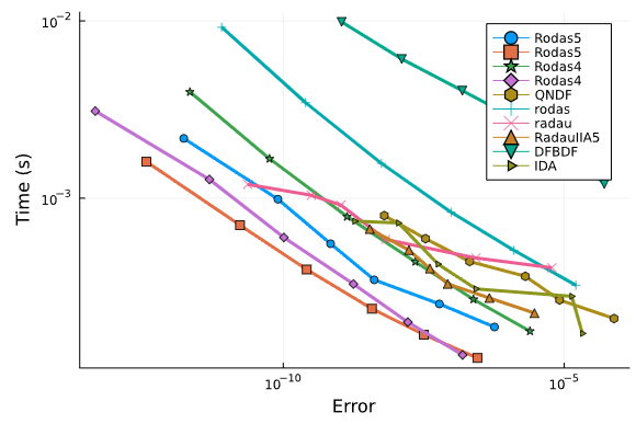
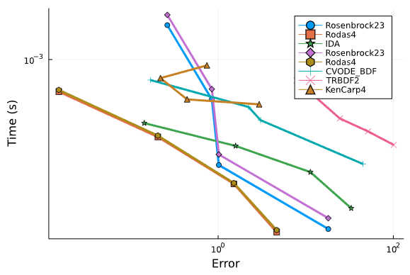
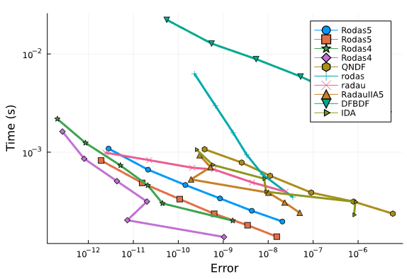
Finally and at last: DAE benchmarks have been added to SciMLBenchmarks.jl! What held us up is that we wanted everything: we wanted to test mass-matrix ODE solvers against fully implicit DAE solvers vs methods which embed the constraints. Given the advancements in ModelingToolkit.jl, we were able to build a code that automatically generates all forms.
Right now we only have a few smaller DAEs implemented, but so far across the board the OrdinaryDiffEq.jl algorithms are outperforming Sundials IDA and DASKR.
Chemical Akzo Nobel:
Orego DAE:
ROBER DAE:
We will continue to expand the suite, and are looking for anyone interested in helping out!
New Documentation Tutorial on Code Optimization for DifferentialEquations
Everyone needs help optimizing their code. Now there is a new tutorial in the DifferentialEquations.jl documentation which goes through non-stiff and stiff ODE codes, showing users how to optimize their code.
Greatly Improved Startup Times
If you haven't been following the big compile time issue, you may have still noticed that things have gotten a lot snappier. We got some very early wins. For example, with non-stiff ODEs, compile times went from almost 5 seconds to about 0.88 seconds:
using OrdinaryDiffEq, SnoopCompile

function lorenz(du,u,p,t)
 du[1] = 10.0(u[2]-u[1])
 du[2] = u[1]*(28.0-u[3]) - u[2]
 du[3] = u[1]*u[2] - (8/3)*u[3]
end

u0 = [1.0;0.0;0.0]
tspan = (0.0,100.0)
prob = ODEProblem(lorenz,u0,tspan)
alg = Tsit5()
tinf = @snoopi_deep solve(prob,alg)

# OrdinaryDiffEq v5.60.2
# InferenceTimingNode: 1.249748/4.881587 on Core.Compiler.Timings.ROOT() with 2 direct children

# Now
# InferenceTimingNode: 0.634172/0.875295 on Core.Compiler.Timings.ROOT() with 1 direct children
For stiff ODEs, we went from 17 seconds to 3 seconds:
function lorenz(du,u,p,t)
 du[1] = 10.0(u[2]-u[1])
 du[2] = u[1]*(28.0-u[3]) - u[2]
 du[3] = u[1]*u[2] - (8/3)*u[3]
end

u0 = [1.0;0.0;0.0]
tspan = (0.0,100.0)

using OrdinaryDiffEq, SnoopCompile
prob = ODEProblem(lorenz,u0,tspan)

alg = Rodas5()
tinf = @snoopi_deep solve(prob,alg)

# Before:
# InferenceTimingNode: 1.460777/16.030597 on Core.Compiler.Timings.ROOT() with 46 direct children

# After:
# InferenceTimingNode: 1.077774/2.868269 on Core.Compiler.Timings.ROOT() with 11 direct children
We fixed issues that invalidated the precompilation improvements with downstream libraries. We even improved compilation times with respect to automatic differentiation:
using OrdinaryDiffEq, SnoopCompile, ForwardDiff

lorenz = (du,u,p,t) -> begin
        du[1] = 10.0(u[2]-u[1])
        du[2] = u[1]*(28.0-u[3]) - u[2]
        du[3] = u[1]*u[2] - (8/3)*u[3]
end

u0 = [1.0;0.0;0.0]; tspan = (0.0,100.0);
prob = ODEProblem(lorenz,u0,tspan); alg = Rodas5();
tinf = @snoopi_deep ForwardDiff.gradient(u0 -> sum(solve(ODEProblem(lorenz,u0,tspan),alg)), u0)
tinf = @snoopi_deep ForwardDiff.gradient(u0 -> sum(solve(ODEProblem(lorenz,u0,tspan),alg)), u0)

# Before:
# First
# InferenceTimingNode: 1.849625/14.538148 on Core.Compiler.Timings.ROOT() with 32 direct children
# Second
# InferenceTimingNode: 1.531660/4.170409 on Core.Compiler.Timings.ROOT() with 12 direct children

# After:
# First
# InferenceTimingNode: 1.181086/3.320321 on Core.Compiler.Timings.ROOT() with 32 direct children
# Second
# InferenceTimingNode: 0.998814/1.650488 on Core.Compiler.Timings.ROOT() with 11 direct children
Across the board most DifferentialEquations.jl usage should be a heck of a lot snappier.
Integro-Differential Equations with NeuralPDE.jl
The NeuralPDE.jl Physics-Informed Neural Network library now supports the automated solution of integro-differential equations.
For example, from a pure symbolic description of a PDE with integrals defined in there:
using NeuralPDE, Flux, ModelingToolkit, GalacticOptim, Optim, DiffEqFlux, DomainSets
import ModelingToolkit: Interval, infimum, supremum

@parameters t
@variables i(..)
Di = Differential(t)
Ii = Integral(t in DomainSets.ClosedInterval(0, t))
eq = Di(i(t)) + 2*i(t) + 5*Ii(i(t)) ~ 1
bcs = [i(0.) ~ 0.0]
domains = [t ∈ Interval(0.0,2.0)]
we can ask the system to generate a neural network representing its solution:
chain = Chain(Dense(1,15,Flux.σ),Dense(15,1))
initθ = Float64.(DiffEqFlux.initial_params(chain))

strategy_ = GridTraining(0.05)
discretization = PhysicsInformedNN(chain,
                                   strategy_;
                                   init_params = nothing,
                                   phi = nothing,
                                   derivative = nothing)
@named pde_system = PDESystem(eq,bcs,domains,[t],[i(t)])
prob = NeuralPDE.discretize(pde_system,discretization)
cb = function (p,l)
    println("Current loss is: $l")
    return false
end
res = GalacticOptim.solve(prob, BFGS(); cb = cb, maxiters=100)
Other and Upcoming Updates
There are many other updates to be aware of which we will highlight in future news posts. As a quick overview:
Massive improvements to ModelingToolkit.jl with mixed discrete+continuous system handling.
GalacticOptim.jl received some major improvements and overhauled documentation over the last round. It now wraps nearly 100 optimization methods from 13 libraries into its common interface.
ExponentialUtilities.jl received a new
exponential!method with greatly improved matrix exponential performance over Julia's Base.PreallocationTools.jl received many cosmetic updates to be easier to use.
Many performance improvements to DiffEqSensitivity.jl and DiffEqFlux.jl
The new library StructuralIdentifiability.jl for computing the structural identifiability of parameters in ODE models will be announced in the next round. A few issues are still being worked out over the next month.
The new library MethodOfLines.jl for automating method of lines discretizations will be announced shortly. Currently it's in a beta mode.
The new library ModelingToolkitStandardLibrary.jl has been created. This will in a beta mode for a bit longer as it fleshes out its offering.
SymbolicNumericIntegration.jl was released and will be included in the next release notes.
MinimallyDisruptiveCurves.jl was released and will be included in the next release notes.