SciML Ecosystem Update: Neural PDEs, Lie Groups, and Stochastic Delay Differential Equations
Another week, another SciML release! Yes, this has been a crazy productive summer so thanks to everyone who has been involved. Let's dive in.
NeuralPDE.jl: Physics-Informed Neural Networks for Automated PDE Solving and High Dimensional PDEs
We have officially released NeuralPDE.jl. This is a domain-specific library for gathering all of the neural network based PDE solver methods. Its main focus are on the two big branches of scientific machine learning:
Physics-informed neural networsk (PINNs)
Forward-Backwards Stochastic Differential Equations for high dimensional PDEs
On the PINN front, the library is all about automated solution of PDEs we want users who have no experience in partial differential equations to be able to slap down a symbolic description of the partial differential equation and get a reasonable result without having to know about details like discretization. To see this in action, let's look at solving the 2-dimensional Poisson equation with this library. We start by describing the PDE:
@parameters x y θ
@variables u(..)
@derivatives Dxx''~x
@derivatives Dyy''~y

# 2D PDE
eq  = Dxx(u(x,y,θ)) + Dyy(u(x,y,θ)) ~ -sin(pi*x)*sin(pi*y)

# Boundary conditions
bcs = [u(0,y,θ) ~ 0.f0, u(1,y,θ) ~ -sin(pi*1)*sin(pi*y),
       u(x,0,θ) ~ 0.f0, u(x,1,θ) ~ -sin(pi*x)*sin(pi*1)]
# Space and time domains
domains = [x ∈ IntervalDomain(0.0,1.0),
           y ∈ IntervalDomain(0.0,1.0)]
Here we described the PDE by its Julia code because, why not: it's as informative and refined as mathematical notation itself! Now let's tell the system to discretize and solve this PDE with a neural network:
dx = 0.1 # Discretization size for sampling purposes
discretization = PhysicsInformedNN(dx)

# Neural network and optimizer
opt = Flux.ADAM(0.02)
dim = 2 # number of dimensions
chain = FastChain(FastDense(dim,16,Flux.σ),FastDense(16,16,Flux.σ),FastDense(16,1))

pde_system = PDESystem(eq,bcs,domains,[x,y],[u])
prob = discretize(pde_system,discretization)
alg = NNDE(chain,opt,autodiff=false)
and then we solve it:
phi,res = solve(prob,alg,verbose=true, maxiters=5000)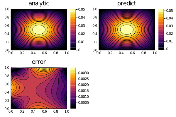
And boom, that's the solution to the PDE. We are continuing to improve this framework, and refactor some of the pieces so that it better connects to more ML and scientific computing library ecosystems, but it's achieving its general goal today so we've decided to release it. Major thanks to @KirillZubov for these developments.
Along with this symbolic form, there are FBSDE methods specifically written for parabolic equations and Kolmogorov backwards equations. This means that high dimensional PDEs that show up in finance, biology, and beyond can now quickly be solved with a neural network. Here's the code to solve a 100 dimensional Hamilton-Jacobi-Bellman equation for LQG optimal control:
using NeuralPDE
using Flux
using DifferentialEquations
using LinearAlgebra
d = 100 # number of dimensions
X0 = fill(0.0f0, d) # initial value of stochastic control process
tspan = (0.0f0, 1.0f0)
λ = 1.0f0

g(X) = log(0.5f0 + 0.5f0 * sum(X.^2))
f(X,u,σᵀ∇u,p,t) = -λ * sum(σᵀ∇u.^2)
μ_f(X,p,t) = zero(X)  # Vector d x 1 λ
σ_f(X,p,t) = Diagonal(sqrt(2.0f0) * ones(Float32, d)) # Matrix d x d
prob = TerminalPDEProblem(g, f, μ_f, σ_f, X0, tspan)
hls = 10 + d # hidden layer size
opt = Flux.ADAM(0.01)  # optimizer
# sub-neural network approximating solutions at the desired point
u0 = Flux.Chain(Dense(d, hls, relu),
                Dense(hls, hls, relu),
                Dense(hls, 1))
# sub-neural network approximating the spatial gradients at time point
σᵀ∇u = Flux.Chain(Dense(d + 1, hls, relu),
                  Dense(hls, hls, relu),
                  Dense(hls, hls, relu),
                  Dense(hls, d))
pdealg = NNPDENS(u0, σᵀ∇u, opt=opt)
@time ans = solve(prob, pdealg, verbose=true, maxiters=100, trajectories=100,
                            alg=EM(), dt=1.2, pabstol=1f-2)
Boom: that's all there is to it. Check out the documentation for more details. There's still a lot of active development here so if you're a student who's interested in this topic, please get in touch.
Lie Group Integrators: Magnus, Runge–Kutta–Munthe-Kaas, and Crouch–Grossman Methods
There are many differential equations which specifically fall under the form of u' = A(t)u, or u' = A(u)u. In these cases, you have geometric properties, like Lie groups, that you can exploit in the solution of the ODE. These Lie group methods are commonly embedded in domain-specific software, usually in robotics, so they are not generally seen except by practitioners of specific scientific areas trying to get the most robust and performant methods in these cases.
Well, SciML wants the most robust and performant methods, so we have now included these methods as part of the standard DifferentialEquations.jl suite thanks to Biswajit Ghosh (@Biswajitghosh98) and Major League Hacking (MLH). To use these methods, you have to define your ODE via a DiffEqOperator. For example:
function update_func(A,u,p,t)
    A[1,1] = cos(t)
    A[2,1] = sin(t)
    A[1,2] = -sin(t)
    A[2,2] = cos(t)
end
A = DiffEqArrayOperator(ones(2,2),update_func=update_func)
prob = ODEProblem(A, ones(2), (1.0, 6.0))
sol = solve(prob,MagnusGL6(),dt=1/10)
that is a quick and easy way to utilize a 6th order Magnus integrator for the u' = A(t)u equation. We have high order methods and adaptive methods, and these all utilize as much mutation as possible to try and be efficient. There's still some optimization that can be done, but the methods are well-tested for correctness and ready to be used where you see fit!
Stochastic Delay Differential Equations and Stochastic Differential-Algebraic Equations
It's finally here! A lot of people had found our ENOC 2020 paper on StochasticDelayDiffEq.jl, but we had to spend some time getting the library to our continuous integration testing and documentation standard before releasing. Well, now it's finally here. StochasticDelayDiffEq.jl allows for solving stochastic differential equations with delayed components and includes higher order and adaptive integrators. It's built on StochasticDiffEq.jl so the methods that you know and love have been transferred to this new domain. It uses all of the development from DelayDiffEq.jl to give robust SDDE solving. SDDEs are very difficult equations to solve, but we try to make it as efficient as possible. Thanks to everyone who was involved, including Henrik Sykora (@HTSykora), for making this possible. For the reveal, here's an SDDE solved with a Milstein method with adaptive time stepping:
function hayes_modelf(du,u,h,p,t)
    τ,a,b,c,α,β,γ = p
    du .= a.*u .+ b .* h(p,t-τ) .+ c
end
function hayes_modelg(du,u,h,p,t)
    τ,a,b,c,α,β,γ = p
    du .= α.*u .+ γ
end
h(p,t) = (ones(1) .+ t);
tspan = (0.,10.)

pmul = [1.0,-4.,-2.,10.,-1.3,-1.2, 1.1]
padd = [1.0,-4.,-2.,10.,-0.0,-0.0, 0.1]

prob = SDDEProblem(hayes_modelf, hayes_modelg, [1.], h, tspan, pmul; constant_lags = (pmul[1],));
sol = solve(prob,RKMil())
In this same vein, SDAEs are possible via singular mass matrices. These have proper testing and now have the official release along with documentation in the latest docs.
With these two announcements, note that because the SciML software composes, you can solve SDDAEs. And yes, these are compatible with neural networks and DiffEqFlux. Go have fun.
Automated Ensemble Parallelism and Multiple GPUs in DiffEqFlux
You can now mix ensemble parallelism, and thus multi-GPU computation, with DiffEqFlux and reverse-mode automatic differentiation. An example of the multithreaded computation of an ensemble which is then trained is as follows:
using OrdinaryDiffEq, DiffEqSensitivity, Flux, Test
pa = [1.0]
u0 = [3.0]

function model2()
  prob = ODEProblem((u, p, t) -> 1.01u .* p, u0, (0.0, 1.0), pa)

  function prob_func(prob, i, repeat)
    remake(prob, u0 = 0.5 .+ i/100 .* prob.u0)
  end

  ensemble_prob = EnsembleProblem(prob, prob_func = prob_func)
  sim = solve(ensemble_prob, Tsit5(), EnsembleThreads(), saveat = 0.1, trajectories = 100).u
end
loss() = sum(abs2,[sum(abs2,1.0.-u) for u in model2()])

pa = [1.0]
u0 = [3.0]
opt = ADAM(0.1)
println("Starting to train")
l1 = loss()
Flux.@epochs 10 Flux.train!(loss, params([pa,u0]), data, opt; cb = cb)
l2 = loss()
@test 10l2 < l1
Major performance improvements to parallelized extrapolation methods
Thanks to Utkarsh (@utkarsh530), we now have fast parallelized implicit extrapolation in OrdinaryDiffEq.jl. You'll find these in the documentation as ImplicitEulerExtrapolation, ImplicitDeuflhardExtrapolation, and ImplicitHairerWannerExtrapolation. For those ODE-inclined, these are pure Julia implementations of SEULEX and SODEX which include automated multithreaded parallelization of the f calls.
New surrogates: Gradient-Enhanced Kriging
Surrogates.jl continues to march forward. If you have not seen the documentation recently, do check it out as it has undergone many major improvements, including showing differences between surrogates on many benchmark problems. One of the latest enhancements is Gradient-Enhanced Kriging, which is an extension to Kriging that can utilize derivative information (from automatic differentiation) to improve the convergence of the surrogate with less samples. Thank Ludovico Bessi (@ludoro) for driving this surrogate project.
Next Directions
The next directions are going to be highly tied to the directions that we are going with the latest Google Summer of Code, so here are a few things to look forward to:
Higher efficiency low-storage Runge-Kutta methods with a demonstration of optimality in a large-scale climate model (!!!).
Continued improvements to parallel and sparse automatic differentiation.
More SDE solvers and adjoints
More performance