SciML Ecosystem Update: Chemical Reaction Modeling and Major Stochastic Simulation Improvements
This ecosystem update has a lot of stochastic components added. We have a new DSL and a bunch of new solvers which incorporate jump dynamics for Levy processes (jump diffusions). Let's "jump" right in!
Catalyst.jl: Chemical Reaction Models
Catalyst.jl is our rebranding of the old DiffEqBio for its expanded role in chemical reaction modeling. You can easily design reaction networks and then simulate them with fast methods for jump equations:
using Catlayst, DiffEqJump

rs = @reaction_network begin
  c1, S + E --> SE
  c2, SE --> S + E
  c3, SE --> P + E
end c1 c2 c3
p = (0.00166,0.0001,0.1)   # [c1,c2,c3]
tspan = (0., 100.)
u0 = [301., 100., 0., 0.]  # [S,E,SE,P]

# solve JumpProblem
dprob = DiscreteProblem(rs, u0, tspan, p)
jprob = JumpProblem(rs, dprob, Direct())
jsol = solve(jprob, SSAStepper())
plot(jsol,lw=2,title="Gillespie: Michaelis-Menten Enzyme Kinetics")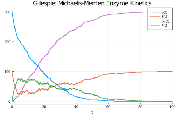
All of the current DifferentialEquations simulation features can be directly applied to Catalyst. Additionally, Catalyst is built on ModelingToolkit.jl so all of the automatic optimization and parallelism features can be directly applied to Catalyst generated code. A lot of the following features also extend continuous-time Markov models as well in new ways!
Adaptive Post-Leap Tau Leaping
Adaptive post-leap tau-leaping is here! For example, an adaptive tau-leaping SIR can be written as:
using StochasticDiffEq, DiffEqJump, DiffEqBase, Statistics
using Test, LinearAlgebra

function regular_rate(out,u,p,t)
    out[1] = (0.1/1000.0)*u[1]*u[2]
    out[2] = 0.01u[2]
end

const dc = zeros(3, 2)
dc[1,1] = -1
dc[2,1] = 1
dc[2,2] = -1
dc[3,2] = 1

function regular_c(du,u,p,t,counts,mark)
    mul!(du,dc,counts)
end

rj = RegularJump(regular_rate,regular_c,2)
jumps = JumpSet(rj)
iip_prob = DiscreteProblem([999.0,1,0],(0.0,250.0))
jump_iipprob = JumpProblem(iip_prob,Direct(),rj)
@time sol = solve(jump_iipprob,TauLeaping())
This is compatible with all of the other parts of DifferentialEquations.jl like event handling, ensemble simulations, and more.
Jump Diffusion Euler-Maruyama and Implicit Euler-Maruyama
Continuing with the theme of jump equations, Euler-Maruyama and Implicit Euler-Maruyama are now compatible with JumpProblem definitions, meaning that equations like jump diffusions can now be directly solved with non-adaptive jumps via Poisson additions. In the following we see the same discrete-jump SIR model, now with Euler-Maruyama:
function rate_oop(u,p,t)
    [(0.1/1000.0)*u[1]*u[2],0.01u[2]]
end

function regular_c(u,p,t,counts,mark)
    dc*counts
end

rj = RegularJump(rate_oop,regular_c,2)
foop(u,p,t) = [0.0,0.0,0.0]
goop(u,p,t) = [0.0,0.0,0.0]
oop_sdeprob = SDEProblem(foop,goop,[999.0,1,0],(0.0,250.0))
jumpdiff_prob = JumpProblem(oop_sdeprob,Direct(),rj)
@time sol = solve(jumpdiff_prob,EM();dt=1.0)
Now you see that there's f and g ready to be changed to mix and match continuous and discrete stochastic behaviors. This is an extension of our previous jump diffusion support by incorporating non-adapted jumping, allowing for scaling to jumps with higher rates.
Adjoints of Stochastic Differential Equations and new SDE Fitting Tutorials
Stochastic differential equations now have adjoint definitions defined which have extra optimizations on diagonal noise SDEs. This extends a comparatively high performing SDE solver to have low-memory SDE fitting. A new tutorial in DiffEqFlux demonstrates how to recover the parameters of an SDE with just a few minutes of compute. Thank @frankschae for this advance!
Tons of methods for high weak order solving of SDEs
Due once again to @frankschae, we have plenty of new high weak order methods for fast solving of SDEs. When paired with recent performance improvements of DiffEqGPU, we see some massive performance advantages for fitting expectations of equations. Formal benchmarks will come soon!
Continuous Normalizing Flows and FFJORD Layers
DiffEqFlux now provides pre-built continuous normalizing flow and FFJORD layers for doing common neural ODE based machine learning. A new tutorial demonstrates how to get up and running with these layers in just a matter of minutes. This brings a system demonstrated to have a 100x neural ODE training advantage over PyTorch into the land of continuous normalizing flow modeling. Thank Diogo Netto (@d-netto) and Avik Pal (@avik-pal) for these strong contributions to the SciML ecosystem!
Sparse Matrix Support in ODE/SDE/DAE Adjoints
The whole SciML ecosystem has already been making use of automated sparsity tooling and now it has improved. Now automated sparse differentiation is performed in the backpass of a differential equation adjoint system using the derived sparsity patterns. This greatly accelerates adjoints of stiff equations, like large partial differential equations. All that is required is for sparse differentiation to be used for the forward solve and the system will kick in and automatically derive and apply it to the reverse.
Next Directions: Google Summer of Code
The next directions are going to be highly tied to the directions that we are going with the latest Google Summer of Code, so here are a few things to look forward to:
Some tooling for automated training of physics-informed neural networks (PINNs) from ModelingToolkit symbolic descriptions of the PDE.
More Lie Group integrator methods.
Higher efficiency low-storage Runge-Kutta methods with a demonstration of optimality in a large-scale climate model (!!!).
More high weak order methods for SDEs
Causal components in ModelingToolkit
And many many more. There will be enough that I don't think we will wait a whole month for the next update, so see you soon!