SciML Ecosystem Update: Auto-Parallelism and Component-Based Modeling
Another month and another set of SciML updates! This month we have been focusing a lot on simplifying our interfaces and cleaning our tutorials. We can demonstrate that no user-intervention is required for adjoints. Also, the ModelingToolkit.jl symbolic modeling language has really come into fruition, allowing component-based models and automated parallelism. Indeed, let's jump right into an example.
ModelingToolkit DAEs and Component-Based Modeling
ModelingToolkit.jl has added the ability to build differential-algebraic equations through acausal component-based models. As an example, let's say we built two Lorenz equations:
using ModelingToolkit, OrdinaryDiffEq

@parameters t σ ρ β
@variables x(t) y(t) z(t)
@derivatives D'~t

eqs = [D(x) ~ σ*(y-x),
       D(y) ~ x*(ρ-z)-y,
       D(z) ~ x*y - β*z]

lorenz1 = ODESystem(eqs,name=:lorenz1)
lorenz2 = ODESystem(eqs,name=:lorenz2)
We can then define an implicit equation that couples the two equations together and solve the system:
@variables a
@parameters γ
connections = [0 ~ lorenz1.x + lorenz2.y + a*γ]
connected = ODESystem(connections,t,[a],[γ],systems=[lorenz1,lorenz2])

u0 = [lorenz1.x => 1.0,
      lorenz1.y => 0.0,
      lorenz1.z => 0.0,
      lorenz2.x => 0.0,
      lorenz2.y => 1.0,
      lorenz2.z => 0.0,
      a => 2.0]

p  = [lorenz1.σ => 10.0,
      lorenz1.ρ => 28.0,
      lorenz1.β => 8/3,
      lorenz2.σ => 10.0,
      lorenz2.ρ => 28.0,
      lorenz2.β => 8/3,
      γ => 2.0]

tspan = (0.0,100.0)
prob = ODEProblem(connected,u0,tspan,p)
sol = solve(prob,Rodas5())

using Plots; plot(sol,vars=(a,lorenz1.x,lorenz2.z))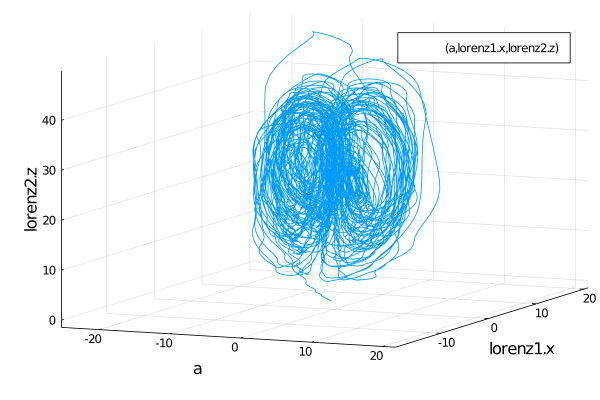
Because of this, one can build up independent components and start tying them together to make large complex models. We plan to start building a comprehensive model library to help users easily generate large-scale models.
ModelingToolkit Compiler targets: C, Stan, and MATLAB
We have added the ability to specify compiler targets from ModelingToolkit. If you have a model specified in its symbolic language, it can generate code for C, Stan, and MATLAB. For example, take the Lotka-Volterra equations:
using ModelingToolkit, Test
@parameters t a
@variables x(t) y(t)
@derivatives D'~t
eqs = [D(x) ~ a*x - x*y,
       D(y) ~ -3y + x*y]
Let's say we now need to deploy this onto an embedded system which only has a C compiler. We can have ModelingToolkit.jl generate the required C code:
ModelingToolkit.build_function(eqs,[x,y],[a],t,target = ModelingToolkit.CTarget()) ==which gives:
void diffeqf(double* internal_var___du, double* internal_var___u, double* internal_var___p, t) {
  internal_var___du[1] = internal_var___p[1] * internal_var___u[1] - internal_var___u[1] * internal_var___u[2];
  internal_var___du[2] = -3 * internal_var___u[2] + internal_var___u[1] * internal_var___u[2];
}
Now let's say we needed to use Stan for some probabilistic programming. That's as simple as:
ModelingToolkit.build_function(eqs,convert.(Variable,[x,y]),convert.(Variable,[a]),t,target = ModelingToolkit.StanTarget()) ==which gives:
real[] diffeqf(real t,real[] internal_var___u,real[] internal_var___p,real[] x_r,int[] x_i) {
  real internal_var___du[2];
  internal_var___du[1] = internal_var___p[1] * internal_var___u[1] - internal_var___u[1] * internal_var___u[2];
  internal_var___du[2] = -3 * internal_var___u[2] + internal_var___u[1] * internal_var___u[2];
  return internal_var___du;
}
When you mix this with the fact that code can automatically be converted to ModelingToolkit, this gives a way to transpile mathematical model code from Julia to other languages, making it easy to develop and test models in Julia and finally transpile and recompile the final model for embedded platforms. However, this automatic transformation can be used in another way...
ModelingToolkit Automatic Parallelism
ModelingToolkit now has automatic parallelism on the generated model code. As an example, let's automatically translate a discretized partial differential equation solver code into ModelingToolkit form:
using ModelingToolkit, LinearAlgebra, SparseArrays

# Define the constants for the PDE
const α₂ = 1.0
const α₃ = 1.0
const β₁ = 1.0
const β₂ = 1.0
const β₃ = 1.0
const r₁ = 1.0
const r₂ = 1.0
const _DD = 100.0
const γ₁ = 0.1
const γ₂ = 0.1
const γ₃ = 0.1
const N = 8
const X = reshape([i for i in 1:N for j in 1:N],N,N)
const Y = reshape([j for i in 1:N for j in 1:N],N,N)
const α₁ = 1.0.*(X.>=4*N/5)

const Mx = Tridiagonal([1.0 for i in 1:N-1],[-2.0 for i in 1:N],[1.0 for i in 1:N-1])
const My = copy(Mx)
Mx[2,1] = 2.0
Mx[end-1,end] = 2.0
My[1,2] = 2.0
My[end,end-1] = 2.0

# Define the discretized PDE as an ODE function
function f!(du,u,p,t)
   A = @view  u[:,:,1]
   B = @view  u[:,:,2]
   C = @view  u[:,:,3]
  dA = @view du[:,:,1]
  dB = @view du[:,:,2]
  dC = @view du[:,:,3]
  mul!(MyA,My,A)
  mul!(AMx,A,Mx)
  @. DA = _DD*(MyA + AMx)
  @. dA = DA + α₁ - β₁*A - r₁*A*B + r₂*C
  @. dB = α₂ - β₂*B - r₁*A*B + r₂*C
  @. dC = α₃ - β₃*C + r₁*A*B - r₂*C
end
Now let's symbolically calculate the sparse Jacobian of the function f!. We can do so by tracing with the ModelingToolkit variables:
@variables du[1:N,1:N,1:3] u[1:N,1:N,1:3] MyA[1:N,1:N] AMx[1:N,1:N] DA[1:N,1:N]
f!(du,u,nothing,0.0)
jac = sparse(ModelingToolkit.jacobian(vec(du),vec(u),simplify=false))
Now that we've automatically translated this into the symbolic system and calculated the sparse Jacobian, we can tell it to generate an automatically multithreaded Julia code:
multithreadedjac = eval(ModelingToolkit.build_function(vec(jac),u,multithread=true)[2])The output is omitted since it is quite large, but the massive speedup over the original form since the sparsity pattern has been automatically computed and an optimal sparse multithreaded Jacobian function has been generated for use with DifferentialEquations.jl, NLsolve.jl, and whatever other mathematical library you wish to use it with.
Indeed, this gives about a 4x speedup on a computer with 4 threads, exactly as you'd expect.
Highlight: sir-julia Model Simulation and Inference Repository
Simon Frost, Principal Data Scientist at Microsoft Health, published an epidemic modeling recipes library, sir-julia which heavily features SciML and its tooling. There are many aspects to note, including integration with probabilistic programming for Bayesian inference. Indeed, the use of DifferentialEquations.jl inside of a Turing.jl macro is simply to use solve inside of the Turing library: no special tricks or techniques required. For example, this looks like:
@model bayes_sir(y) = begin
  # Calculate number of timepoints
  l = length(y)
  i₀  ~ Uniform(0.0,1.0)
  β ~ Uniform(0.0,1.0)
  I = i₀*1000.0
  u0=[1000.0-I,I,0.0,0.0]
  p=[β,10.0,0.25]
  tspan = (0.0,float(l))
  prob = ODEProblem(sir_ode!,
          u0,
          tspan,
          p)
  sol = solve(prob,
              Tsit5(),
              saveat = 1.0)
  sol_C = Array(sol)[4,:] # Cumulative cases
  sol_X = sol_C[2:end] - sol_C[1:(end-1)]
  l = length(y)
  for i in 1:l
    y[i] ~ Poisson(sol_X[i])
  end
end;
For more examples, please consult the repository which is chock full of training examples. However, this demonstration leads us to your next major release note:
The End of concrete_solve
It's finally here: concrete_solve has been deprecated for, you guessed it, solve. If you want to solve an ODE with Tsit5(), how do you write it?
solve(prob,Tsit5())If you want to differentiate the solution to an ODE with Tsit5(), how do you write it?
solve(prob,Tsit5())If you want to use Bayesian inference on Tsit5() solutions, how do you write it?
solve(prob,Tsit5())That is correct: for both forward and reverse mode automatic differentiation, there is no modification that is required. When forward-mode automatic differentiation libraries are used, type handling will automatically promote to ensure the solution is differentiated properly. When reverse-mode automatic differentiation is used, the backpropogation will automatically be replaced with adjoint sensitivity methods which can be controlled through the sensealg keyword argument. The result is full performance and flexibility, but no code changes required.
This is a step up from where we were. In the first version of DiffEqFlux.jl, we required the use of special functions like diffeq_adjoint to use the adjoint methods. Then we better integrated by having concrete_solve, which was a neutered version of solve but would work perfectly in the AD contexts. Now, solve does it all, and so there is no other function to use.
Demonstration: Stiff Neural ODE with Nested Forward, Reverse, and Adjoint AD
As a quick demonstration, here's the use of checkpointed interpolating adjoints over a stiff ODE solver.
using OrdinaryDiffEq, Flux, DiffEqSensitivity
model = Chain(Dense(2, 50, tanh), Dense(50, 2))
p, re = Flux.destructure(model)
dudt!(u, p, t) = re(p)(u)
u0 = rand(2)
odedata = rand(2,11)
function loss()
  prob = ODEProblem(dudt!, u0, (0.0,1.0), p)
  my_neural_ode_prob = solve(prob, RadauIIA5(), saveat=0.1)
  sum(abs2,my_neural_ode_prob .- odedata)
end
loss()
Flux.gradient(loss,Flux.params(u0,p))
Note that it's nesting 3 modes of differentiation all in the optimal ways: forward-mode for the Jacobians in the stiff ODE solver, an adjoint mode for the derivative of solve, and reverse-mode for the vector-Jacobian-product (vjp) calculation of the neural network. This means that the DiffEqFlux.jl library is pretty much at its endgame where nothing about your code needs to be changed to utilize its tools!
Next Directions: Google Summer of Code
The next directions are going to be highly tied to the directions that we are going with the latest Google Summer of Code, so here are a few things to look forward to:
Adjoints of stochastic differential equations. Just like with ODEs, adjoint sensitivity methods for SDEs are being integrated into the library and are being setup to be automatically used when performing reverse mode automatic differentiation over
solve. Actually, one of these methods is already completed, but we will be rounding out the offering a bit before documenting and formally releasing it. Be on the lookout for some pretty major neural SDE improvements.Some tooling for automated training of physics-informed neural networks (PINNs) from ModelingToolkit symbolic descriptions of the PDE.
Efficiency enhancements to native Julia BDF methods.
More Lie Group integrator methods.
Higher efficiency low-storage Runge-Kutta methods with a demonstration of optimality in a large-scale climate model (!!!).
More high weak order methods for SDEs
Causal components in ModelingToolkit
And many many more. There will be enough that I don't think we will wait a whole month for the next update, so see you soon!