A "Jupyter" of DiffEq: Introducing Python and R Bindings for DifferentialEquations.jl
Differential equations are used for modeling throughout the sciences from astrophysical calculations to simulations of biochemical interactions. These models have to be simulated numerically due to the complexity of the resulting equations. However, numerical solving differential equations presents interesting software engineering challenges. On one hand, speed is of utmost importance. PDE discretizations quickly turn into ODEs that take days/weeks/months to solve, so reducing time by 5x or 10x can be the difference between a doable and an impractical computation. But these methods are difficult to optimize in a higher level language since a lot of the computations are small, hard to vectorize loops with a user-defined function directly in the middle (one SciPy developer described it as a "worst case scenario for Python") . Thus higher level languages and problem-solving environments have resorted to a strategy of wrapping C++ and Fortran packages, and as described in a survey of differential equation solving suites, most differential equation packages are wrapping the same few methods.
While this strategy works, efficiency in this field is not just due to the engineering practices. There is no perfect method across the whole range of differential equations. Each type of differential equation has different qualities that need to be taken advantage of in order to have an efficient solver. There are hundreds of methods to choose from, many of which do not have a classical canonical implementation (or any!), with some making use of semi-linearity, partial stiffness, etc. of the equation. Additionally, recent scientific models have been growing in realism, meaning that the ability to efficiently handle problems like stochastic differential equations, delay differential equations, and differential-algebraic equations are growing in importance. Thus the ability to build software in a productive manner is also required (a task that is usually relegated to high level scripting languages!).
However, the software development area of the field has not been keeping up with the changing waves of science and many of the greats who built the classic C++/Fortran infrastructure, such as Alan Hindmarsh and Lawrence Shampine, have now retired. But it's been hard to get new people into open source development because software development is not seen as a valuable research product for academics, which is an issue that has pushed people out of academic careers. It has been mentioned that "every great open source math library is built on the ashes of someone's academic career". What we needed was a new way to connect software development to the mathematics so that we can get the newest/fastest methods into the hands of those who need them while keeping in line with academic incentives (publications and grants).
The Goal of the Organization: Help Researchers Connect Code with Users
There were three problems which really needed to be addressed back when SciML was started:
How do we condense the mountain of recent methods research into a "solve this" button for scientific domain experts?
How do we give power users the flexibility to solve equations as efficiently as possible?
How do we gather the methods of the field so that way usable and precise benchmarks can guide the theoretical development?
As both the efficiency and complexity of the methods grow, it is important that we address (1) and allow for people who specialize in scientific models to be able to solve their problems without having to become numerical methods and software development experts. This requires that new methods, like adaptivity for stochastic differential equations, proliferate while not increasing the user-burden. But at the same time, the computational physicists and engineers who specialize in solving difficult PDEs fall under (2) and need access to every little detail about Jacobian linear solver choices across the vast field of methods. This level of detail had not traditionally been exposed in the interfaces of higher level languages, so most of this crowed was forced to stay in C++/Fortran. But what methods do you even develop or use? It was interesting to find out that the vast majority of methods have never been benchmarked together or have an easy way to do so! This means that (3) is of utmost importance for guiding the field.
To tackle this problem, we developed a confederated package ecosystem in Julia which has become known as DifferentialEquations.jl. The architecture of the software is described here and it allows for any developers to add dispatches to a common solve function. This ends up being important because it allows researchers to keep their research "their own" in their own repositories while contributing to this common cause. This is required since the researchers developing the methods need the research outputs to grow their own careers, but at the same it allows us to make use of their newest methods in more complex software. By doing so, we strike a balance between the user and research communities which is required to keep iterating the software of the field. [Note: we will be releasing a paper in a special issue which discusses exactly how this was done in further detail.]
At this point we can say this methodology has been successful. We have a large active community, SciML, which is devoted to solving the user and theoretical problems of the field through software development. The organization continually fields a large number of student researchers (and Google Summer of Code developers). We have covered areas which have traditionally not had adequate open-source software with high performance implementations, such as symplectic integrators, exponential and IMEX integrators, and high order adaptive Runge-Kutta methods for SDEs. These solvers then automatically compose with higher level tools for things like parameter estimation and chemical reaction modeling.
Now that we have a successful and growing software ecosystem, it makes sense to cast our nets as wide as possible and distribute our methods to all of the users that need them. The software was developed in Julia because of its unique ability to hit our efficiency and productivity demands. However, we recognize that we live in a poly-language world and so in order to really meet the goals of our organization, we need to expand and become multi-language compatible.
Introducing diffeqpy and diffeqr
To meet the multi-language demands, we have produced the diffeqpy and diffeqr packages for Python and R respectively. Our focus was on addressing (1) and (2): giving domain-experts high efficiency automated tooling and giving the bindings the required flexibility to be tweaked to efficiency. Let me state that we are not all the way there yet, this is still very new, but we have made major headway. I think the best way to show what we've done is to show some examples.
(Just for reference, "Jupyter" in Jupyter notebooks stands for Julia+Python+R. The title is punning off of that, but we aren't associated with the Jupyter notebook.)
Interface Matching: Differential-Algebraic Equations
As a first example, let's solve the Robertson differential-algebraic equation (DAE) in each of the languages. A DAE is an ODE defined implicitly: . These are interesting because it allows constraints to be incorporated as part of the equation. The Robertson equation is defined as follows:
In DifferentialEquations.jl, we would solve this equation by defining that implicit system via its residual, and calling solve:
function f(resid,du,u,p,t)
  resid[1] = - 0.04u[1]              + 1e4*u[2]*u[3] - du[1]
  resid[2] = + 0.04u[1] - 3e7*u[2]^2 - 1e4*u[2]*u[3] - du[2]
  resid[3] = u[1] + u[2] + u[3] - 1.0
end
u₀ = [1.0, 0, 0]
du₀ = [-0.04, 0.04, 0.0]
tspan = (0.0,100000.0)
using DifferentialEquations
differential_vars = [true,true,false]
prob = DAEProblem(f,du₀,u₀,tspan,differential_vars=differential_vars)
sol = solve(prob)
using Plots; plotly() # Using the Plotly backend
plot(sol, xscale=:log10, tspan=(1e-6, 1e5), layout=(3,1))
This code directly translates over to Python with diffeqpy by putting "de." in front of package functions:
from diffeqpy import de

def f(resid,du,u,p,t):
    resid[0] = - 0.04*u[0] + 1e4*u[1]*u[2] - du[0]
    resid[1] = + 0.04*u[0] - 3e7*u[1]**2 - 1e4*u[1]*u[2] - du[1]
    resid[2] = u[0] + u[1] + u[2] - 1.0
    return

u0 = [1.0, 0, 0]
du0 = [-0.04, 0.04, 0.0]
tspan = (0.0,100000.0)
differential_vars = [True,True,False]
prob = de.DAEProblem(f,du0,u0,tspan,differential_vars=differential_vars)
sol = de.solve(prob)
The R interface is similar:
de <- diffeqr::diffeq_setup()

f <- function (du,u,p,t) {
  resid1 = - 0.04*u[1]              + 1e4*u[2]*u[3] - du[1]
  resid2 = + 0.04*u[1] - 3e7*u[2]^2 - 1e4*u[2]*u[3] - du[2]
  resid3 = u[1] + u[2] + u[3] - 1.0
  c(resid1,resid2,resid3)
}
u0 <- c(1.0, 0, 0)
du0 <- c(-0.04, 0.04, 0.0)
tspan <- c(0.0,100000.0)
differential_vars <- c(TRUE,TRUE,FALSE)
prob <- de$DAEProblem(f,du0,u0,tspan,differential_vars=differential_vars)
sol <- de$solve(prob)
udf <- as.data.frame(t(sapply(sol$u,identity)))
plotly::plot_ly(udf, x = sol$t, y = ~V1, type = 'scatter', mode = 'lines') |>
  plotly::add_trace(y = ~V2) |>
  plotly::add_trace(y = ~V3)
Notice that the interfaces are virtually identical. Even key features about the solution are preserved. For example, the return sol is a continuous function sol(t) in Julia. This is true in Python as well. This means that the in-depth documentation carries across languages as well. Even the common solver options carry across languages. For example, in Julia, to decrease the solver tolerances and specify that we want to use the SUNDIALS IDA algorithm we would do:
sol = solve(prob,IDA(),abstol=1e-8,reltol=1e-8)sol = solve(prob,de.IDA(),abstol=1e-8,reltol=1e-8)sol = de$solve(prob,de$IDA(),abstol=1e-8,reltol=1e-8)This interface commonality means the following:
Anyone who has developed an algorithm on the DifferentialEquations.jl common interface automatically gets cross language compatibility!
Remember, the interface is confederated and thus there exists packages outside of the SciML organization which are part of the interface (LSODA.jl is an example). However, due to the dispatch handling of the common interface, these developers get cross language compatibility via the release of diffeqpy and diffeqr.
Over time we will work on getting the R interface more in line with the others.
R and Python JITing: Stochastic Differential Equations (SDEs) with Non-Diagonal Noise
A stochastic differential equation is a problem of the form
where and are vector functions. If we instead use as a matrix function against the vector of Brownian motions (the translation is described in the DifferentialEquations.jl documentation), then we have
where is a matrix. When is a diagonal matrix this is known as diagonal noise. DifferentialEquations.jl started out as a package developed for adaptive integrators for diagonal noise SDEs, and the research has continued in this area, with the newest default methods offering over 6000x speedups over the traditional methods. But instead of diagonal noise, let's take a look at non-diagonal stochastic differential equations.
In this case, of course is non-diagonal. What this means is that different parts of the system share Wiener processes (or more practically, random numbers). This comes up for example when modeling reaction systems arising from Poisson processes, since you can show that the randomness is due to events like chemical reactions and so each chemical of a system should share the same randomness of a reaction. Modeling these correlations correctly can be crucial for reproducing the features of a system.
In DifferentialEquations.jl, you solve such a problem by giving the vector function and the matrix function. You must also define what the matrix is like so that it is known how many random processes there should be. Let's solve the Lorenz equation with two Wiener processes and heavy cross-correlations. This equations is given via:
The code then translates the problem to:
using DifferentialEquations
function f(du,u,p,t)
  du[1] = 10.0*(u[2]-u[1])
  du[2] = u[1]*(28.0-u[3]) - u[2]
  du[3] = u[1]*u[2] - (8/3)*u[3]
end

function g(du,u,p,t)
  du[1,1] = 0.3u[1]
  du[2,1] = 0.6u[1]
  du[3,1] = 0.2u[1]
  du[1,2] = 1.2u[2]
  du[2,2] = 0.2u[2]
  du[3,2] = 0.3u[2]
end

u0 = [1.0,0.0,0.0]
tspan = (0.0,100.0)
nrp = zeros(3,2)
prob = SDEProblem(f,g,u0,tspan,noise_rate_prototype=nrp)
sol = solve(prob)
plot(sol) # And plot the solution
Almost the same code works in diffeqpy, adding "de.":
def f(du,u,p,t):
  x, y, z = u
  sigma, rho, beta = p
  du[0] = sigma * (y - x)
  du[1] = x * (rho - z) - y
  du[2] = x * y - beta * z

def g(du,u,p,t):
  du[0,0] = 0.3*u[0]
  du[1,0] = 0.6*u[0]
  du[2,0] = 0.2*u[0]
  du[0,1] = 1.2*u[1]
  du[1,1] = 0.2*u[1]
  du[2,1] = 0.3*u[1]


u0 = [1.0,0.0,0.0]
tspan = (0.0,100.0)
p = [10.0,28.0,2.66]
nrp = numpy.zeros((3,2))
prob = de.SDEProblem(f,g,u0,tspan,p,noise_rate_prototype=nrp)
jit_prob = de.jit(prob)
sol = de.solve(jit_prob,saveat=0.005)

# Now let's draw a phase plot

us = de.stack(sol.u)
from mpl_toolkits.mplot3d import Axes3D
fig = plt.figure()
ax = fig.add_subplot(111, projection='3d')
ax.plot(us[0,:],us[1,:],us[2,:])
plt.show()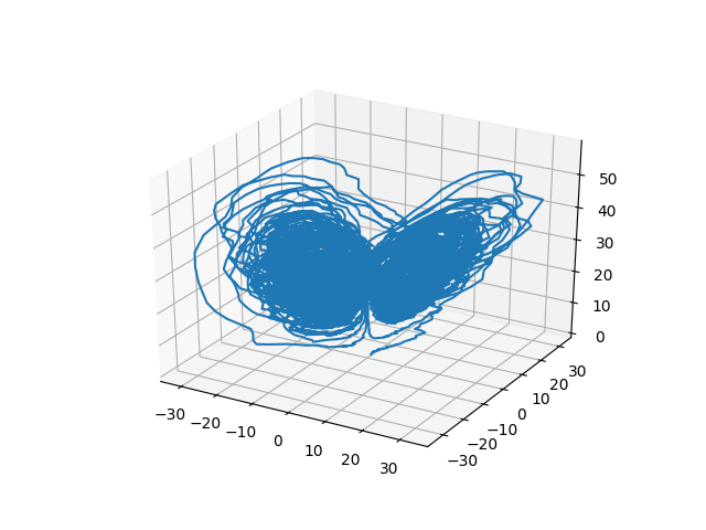
You can clearly see the warping effect of the correlations from this image generated by matplotlib. The same ideas carry over to R:
f <- JuliaCall::julia_eval("
function f(du,u,p,t)
  du[1] = 10.0*(u[2]-u[1])
  du[2] = u[1]*(28.0-u[3]) - u[2]
  du[3] = u[1]*u[2] - (8/3)*u[3]
end")
g <- JuliaCall::julia_eval("
function g(du,u,p,t)
  du[1,1] = 0.3u[1]
  du[2,1] = 0.6u[1]
  du[3,1] = 0.2u[1]
  du[1,2] = 1.2u[2]
  du[2,2] = 0.2u[2]
  du[3,2] = 0.3u[2]
end")
u0 <- c(1.0,0.0,0.0)
tspan <- c(0.0,100.0)
noise_rate_prototype <- matrix(c(0.0,0.0,0.0,0.0,0.0,0.0), nrow = 3, ncol = 2)

JuliaCall::julia_assign("u0", u0)
JuliaCall::julia_assign("tspan", tspan)
JuliaCall::julia_assign("noise_rate_prototype", noise_rate_prototype)
prob <- JuliaCall::julia_eval("SDEProblem(f, g, u0, tspan, p, noise_rate_prototype=noise_rate_prototype)")
sol <- de$solve(prob)
udf <- as.data.frame(t(sapply(sol$u,identity)))
plotly::plot_ly(udf, x = ~V1, y = ~V2, z = ~V3, type = 'scatter3d', mode = 'lines')
Notice that these examples show off that diffeqpy can use functions that are JIT'd by Julia, and diffeqr can directly define functions in Julia to allow for JIT compilation. This JIT compilation from Julia vastly outperforms what can be done with Numba with SciPy. Solving these kinds of nonlinear stochastic differential equations to strong accuracy of 1e-2 is a very difficult and time consuming problem for traditional methods, but the adaptive algorithms along with the function JITing allows these problems to be solved in an entirely automated way, giving domain-experts access to these equations as modeling tools without the burden of developing specialized solvers.
Note that DifferentialEquations.jl allows for all sorts of tweaks on this equation. You can change to algorithms that solve the problem in the Stratonovich sense, utilize a sparse matrix for the noise matrix, etc. So once again, these methods address goals (1) and (2).
Correctness and Accuracy: Delay Differential Equations (DDEs)
Correctness and accuracy can be a very subtle issue for this numerical differential equations. It's deeply mathematical and once you go beyond ODEs to DAEs/SDEs/DDEs you quickly run into difficulties like discontinuities. I pointed out in the big differential equation suite blog post that deSolve's (R) documentation explicitly states that they are using multistep methods without discontinuity tracking in the delay differential equation solvers which is discussed as problematic in DDE solver literature. That isn't meant as a knock on the researchers in any sense, but it's a cautionary note about a very subtle detail in the integration methods which can lead to real inaccuracies. Indeed, this is more showing a systematic problem in academia's relation to open source since the few existing packages tend to be maintained by scientists who need the methods for their research (Thomas Petzoldt of deSolve looks like he has some cool work!) rather than having groups of methods researchers with a long-term dedication to software implementations of methods (and maintenance!). I mean this with no disrespect: it is difficult to continually develop and maintain a software that's not one of your main sources of career progression or funding, yet open source academic software has done quite well despite this limitation!
But because of the infrastructure, methodology expertise, and community around the SciML organization, we can actively implement and maintain the most up-to-date methods and have frequently have open discussions about accuracy and efficiency throughout the repositories. But the main thing is that be congregating numerical differential equation research together, we can keep an active organization with active methods research and researchers (the key here was making it field-specific so we can stay on "the front lines"! We're taking the easy way out and staying close to our field and funding source). With these new language bindings, we can share our knowledge and research across the open source ecosystem, connecting dedicated methods researchers to the users who need the resulting methods. For example, this problem and solution in R shows the discontinuity tracking of a DDE with a constant-time lag, accurately making out the kink at t=20:
f <- JuliaCall::julia_eval("function f(du, u, h, p, t)
  du[1] = 1.1/(1 + sqrt(10)*(h(p, t-20)[1])^(5/4)) - 10*u[1]/(1 + 40*u[2])
  du[2] = 100*u[1]/(1 + 40*u[2]) - 2.43*u[2]
end")
h <- JuliaCall::julia_eval("function h(p, t)
  [1.05767027/3, 1.030713491/3]
end")
u0 <- c(1.05767027/3, 1.030713491/3)
tspan <- c(0.0, 100.0)
constant_lags <- c(20.0)
JuliaCall::julia_assign("u0", u0)
JuliaCall::julia_assign("tspan", tspan)
JuliaCall::julia_assign("constant_lags", tspan)
prob <- JuliaCall::julia_eval("DDEProblem(f, u0, h, tspan, constant_lags = constant_lags)")
sol <- de$solve(prob,de$MethodOfSteps(de$Tsit5()))
udf <- as.data.frame(t(sapply(sol$u,identity)))
plotly::plot_ly(udf, x = sol$t, y = ~V1, type = 'scatter', mode = 'lines') |> plotly::add_trace(y = ~V2)
and Python:
f = de.seval("""
function f(du, u, h, p, t)
  du[1] = 1.1/(1 + sqrt(10)*(h(p, t-20)[1])^(5/4)) - 10*u[1]/(1 + 40*u[2])
  du[2] = 100*u[1]/(1 + 40*u[2]) - 2.43*u[2]
end""")
u0 = [1.05767027/3, 1.030713491/3]

h = de.seval("""
function h(p,t)
  [1.05767027/3, 1.030713491/3]
end
""")

tspan = (0.0, 100.0)
constant_lags = [20.0]
prob = de.DDEProblem(f,u0,h,tspan,constant_lags=constant_lags)
sol = de.solve(prob,saveat=0.1)

u1 = [sol.u[i][0] for i in range(0,len(sol.u))]
u2 = [sol.u[i][1] for i in range(0,len(sol.u))]

import matplotlib.pyplot as plt
plt.plot(sol.t,u1)
plt.plot(sol.t,u2)
plt.show()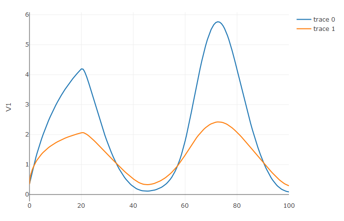
This is a win-win situation for everyone: domain-experts can spend more time (more productively/efficiently) simulating difficult models, while methods researchers can get better feedback about the effectiveness of integrator classes to then better guide the development of the next numerical methods. We have already seen the effects from the Julia ecosystem, with DynamicalSystems.jl and QuantumOptics.jl identifying new issues which have started new research projects!
Performance: Ordinary Differential Equations (ODEs)
Lastly, let's show some ODE solving. Everyone can do ODE solving, so it's only interesting if you can improve on it. So... let's look at timing. Python's SciPy and R's deSolve are just wrapping Fortran/C++ code. We're replacing that C++ and Fortran code with Julia code. The question on your mind must be: can we actually improve upon that?
Well yes, but currently with a caveat. Let's look at some timings. Starting with SciPy, let's use a Numba JIT-compiled derivative function for the Lotka-Volterra equation.
import numpy as np
from scipy.integrate import odeint
import timeit
import numba

def f(u, t, sigma, rho, beta):
    x, y, z = u
    return [sigma * (y - x), x * (rho - z) - y, x * y - beta * z]

u0 = [1.0,0.0,0.0]
tspan = (0., 100.)
t = np.linspace(0, 100, 1001)
sol = odeint(f, u0, t, args=(10.0,28.0,8/3))

def time_func():
    odeint(f, u0, t, args=(10.0,28.0,8/3),rtol = 1e-8, atol=1e-8)

timeit.Timer(time_func).timeit(number=100) # 4.273871208999935

numba_f = numba.jit(f)
def time_func():
    odeint(numba_f, u0, t, args=(10.0,28.0,8/3),rtol = 1e-8, atol=1e-8)

timeit.Timer(time_func).timeit(number=100) # 2.749094666000019
If we replace that with the naïve Julia JIT-compiled function into diffeqpy, it speeds up a lot:
def f(du,u,p,t):
    x, y, z = u
    sigma, rho, beta = p
    du[0] = sigma * (y - x)
    du[1] = x * (rho - z) - y
    du[2] = x * y - beta * z

u0 = [1.0,0.0,0.0]
tspan = (0., 100.)
p = [10.0,28.0,2.66]
prob = de.ODEProblem(f, u0, tspan, p)
fastprob = de.jit(prob)
sol = de.solve(fastprob,saveat=t,abstol=1e-8,reltol=1e-8)

def time_func():
    sol = de.solve(fastprob,saveat=t,abstol=1e-8,reltol=1e-8)

timeit.Timer(time_func).timeit(number=100) # 1.1045269999999618
def time_func():
sol = de.solve(fastprob,de.Tsit5(),saveat=t,abstol=1e-8,reltol=1e-8)
timeit.Timer(time_func).timeit(number=100) # 0.646715709000091If we were using pure-Julia, we could get another 2x-3x out by using StaticArrays.jl. Again, the emphasis here is both the efficiency of the implementation and the method, with the method mattering a lot. SciPy is defaluting to just LSODA here, while diffeqpy is making a choice from 100's of methods, pulling a default based on the characteristics of the problem and the arguments. Even then, we can improve on the defaults by making a smart choice. 10x faster can mean a lot when you're running week long parameter estimations (oops, less than a day now!).
The same story happens in R. With deSolve, we time vode:
chaos <- function(t, state, parameters) {
  with(as.list(c(state)), {
    dx <- -8/3 * x + y * z
    dy <- -10 * (y - z)
    dz <- -x * y + 28 * y - z
    list(c(dx, dy, dz))
  })
}
state <- c(x = 1.0, y = 0.0, z = 0.0)
times <- seq(0, 100, 0.01)
out <- deSolve::vode(state, times, chaos, 0)
system.time(a <- for (i in 1:100){deSolve::vode(state, times, chaos, 0, atol=1e-8, rtol=1e-8)})

user  system elapsed
25.64    0.00   25.83
When using R-defined functions, it doesn't turn out so well:
f <- function(u,p,t) {
  du1 = p[1]*(u[2]-u[1])
  du2 = u[1]*(p[2]-u[3]) - u[2]
  du3 = u[1]*u[2] - p[3]*u[3]
  return(c(du1,du2,du3))
}
u0 <- c(1.0,0.0,0.0)
tspan <- c(0.0,100.0)
p <- c(10.0,28.0,8/3)
prob <- de$ODEProblem(f, u0, tspan, p)
sol <- de$solve(prob)

system.time(a <- for (i in 1:100){de$solve(prob, de$Tsit5(), saveat=times, abstol=1e-8, reltol=1e-8)})

user  system elapsed
153.93    0.14  154.89
But with Julia JIT-compiled functions we do much better:
fastprob <- diffeqr::jitoptimize_ode(de,prob)
sol <- de$solve(fastprob,de$Tsit5())
system.time(a <- for (i in 1:100){de$solve(fastprob, de$Tsit5(), saveat=times, abstol=1e-8, reltol=1e-8)})

user  system elapsed
2.11    0.00    2.12
Again improving timings >10x over the previous C++/Fortran solution. So that's where we're at. Our methods are improvements, but currently the bridges for calling the R/Python defined functions have too much overhead to do well in the inner loop. But diffeqpy and diffeqr are some of the first packages to use these Python->Julia (pyjulia) and R->Julia (JuliaCall) libraries, so hopefully this will spur some development.
Notes
One way we can get around this is to just develop nicer syntax for writing Julia functions. For example, a package like PythonSyntax.jl let's you write a function in Julia using Python syntax and it will auto-convert at macro expansion time.
Also, benchmarking ODE solvers requires taking into account timing and error. Error is related to the (local) tolerance choice but it's not exactly the same. To be rigorous we need to estimate the global error. See DiffEqBenchmarks.jl for comprehensive performance testing between the Julia, Fortran, and C++ packages which shows the (time,error) relationships on a large array of stiff and non-stiff problems.
The Next Steps
Although this is a lot of progress (diffeqr is setup and registered in CRAN, diffeqpy is setup and registered in PyPi), there is still a lot of work to do, including:
We need to get the installation to be smoother. Right now you have to install Julia and DiffEq on your own, then do the R/Python part. It should just be dead simple one step "one-click installs".
We need to get R's interface compatible with the problem/solve format. R's return should be a full solution object instead of just the time and state fields. This will make more features and documentation carry over directly to R.
We need to get auto-differentiation through Python/Numba functions working, or fix the defaults. (Julia's autodiff already works through R functions through Changcheng Li (@Non-Contradiction) 's great work on JuliaCall!)
We need more comprehensive documentation and tutorials in the R and Python languages.
We need to get native Python and R functions wrapped better. Calling a Numba JIT-compiled function should be much better than it is.
And of course there's always more. This release is a working beta. This is the first "major" application of these R->Julia and Python->Julia tools, and I hope this gives a big incentive to Julia developers to make these bridges top notch, along with being a good avenue to demonstrate other tooling like static compilation. In addition, I hope to get in touch with developers from SageMath and PyMC3 so that we can work together towards the common goal of expanding the set of easily available open source tooling. If you have Python/R OSS expertise to donate, we'd love to have you on board! There's a lot of potentially simple issues to solve that just require knowledge of their package ecosystems (install scripts).
Showing Support
To show support for this project, please star the DifferentialEquations.jl, diffeqpy, and diffeqr repositories. These serve as a simple measure of users and community interest which we hope can be utilized to bring in more funding, researchers, and students. please feel free to get in touch with us through the issues, chatroom, or email (just find out how to email Chris Rackauckas or SciML). In addition, we are thankful to the academics who have funded student projects throughout the ecosystem. Also, if you have ideas for projects that can be done and have academic currency (grants or possible publications), please feel free to contact us. If you are an open source project who wishes to make use of this tooling and need help, please feel free to contact us. While we cannot guarantee the ability to help everyone, I hope we can keep putting as much time and energy in as possible, along with growing our developer base.
Please thank Changcheng Li (@Non-Contradiction) and Takafumi Arakaki (@tkf) for being instrumental in getting these packages up and running. We hope this can be a service to the community.